Plots setup
Data can be analyzed and visualized in the software. Both data analysis and visualization of the processed data is set up in a plot.
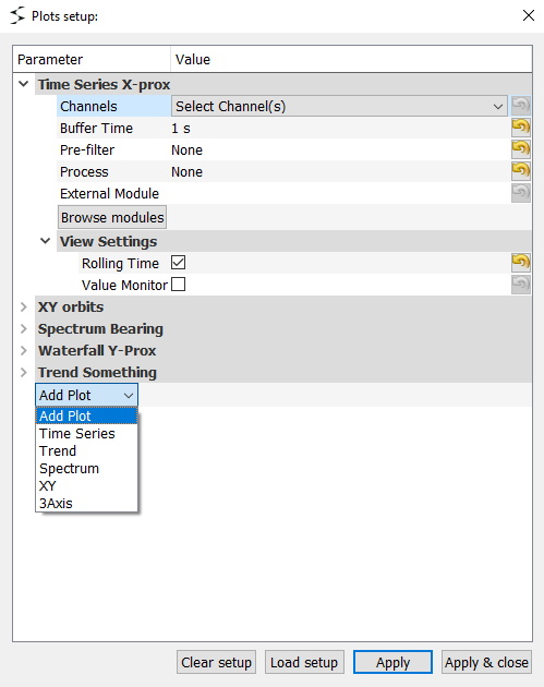
The plots setup dialog is launched via “Setup”->”Plots Setup”. The dialog shows the currently added plots. Each plot can be expanded to reveal the individual settings, which depends on the plot type.

Plots setup dialog
A plot is added by pushing the dropdown “Add plot” and selecting the plot type. Each plot can be renamed or removed by right clicking the plot title. The whole plots setup can be cleared via the “Clear setup” button.
A plots setup can be loaded from a (.sava) setup file by selecting “Load setup”.
Tip
The plot setup for an individual plot can be opened via the context menu in the plot container.
Common plot settings
All plot types have the following settings in common:
Channels
The channels processed/plotted in the plot. If a source is setup, the channels names can be selected from a dropdown. Elsewhere an integer allay (starting at 0), is used to select channels. An empty array selects all channels. By right clicking the channel box, one can “select all”, “deselect all” or “reset the order”. The order is matters for some plot types.
Pre filtering
Time domain filtering before any other processing is applied. Currently only N’t Order Butter filter is available.
View settings
The view settings can be altered while the source is running, without clearing the already processed values. If the value monitor is checked, the graphical visualization is disabled, and only the latest value(s) are displayed as a float.
Tip
A plots view settings are accessible directly in plot the context menu, see plot container.
External process module
The software is able to load a custom Python script and use it an external process module. This can be utilized to set up custom processes or forward data to external application etc.
Select a file by either entering the path in “External module” or browse for the file, by pushing “Browse modules”. The path can be absolute or relative (to current directory).
Note
Examples of external process modules (“extProcessModule.py” and “extProcessModuleXY.py”) are located at: “Help”->”External Module Examples”.
Plot types
Time Series
For sampled data points vs time plots. Primarily used for displaying raw data.
Settings:
Buffer time: Time samples stored in moving buffer and displayed simultaneously
Process: Processing of raw data:
None: Raw data
Order tracking: Filtered raw data via order tracking (see processing types)
Trend
For trending, a downsampled representation, of sampled data vs time plots.
Settings:
Trend time: Time samples in each trend bin. Will also be time between samples in the plot.
Trend type:
Mean: The mean of the samples in the bin
Peak-Peak: Difference between larges and smallest value in the bin
0-Peak: Half Peak-Peak
Min/Max: The minimum/maximum value in the bin
Abs max: The maximum absolute value in the bin
RMS: Root Mean Square value of the bin. Also called “Effective value” of “Vibration energy” of a signal.
Variance: A measure of the AC Power of the samples in the bin
Kurtosis: A measure of the distribution of the samples in the bin, in relation to normal distribution (Kurtosis==3)
Skew: A measure of the distribution symmetry of the samples in the bin.
MAD: Mean Absolute Deviation of the bin
Tacho: See processing types
Order tracking: See processing types
Spectrum
For sampled data (magnitude and/or phase) in the frequency domain plots.
Settings:
Type: FFT or FRF (see processing types)
N Lines: Number of samples in each bin
Window: Windowing of the sig FFT
Overlap: Overlap of bins
N Averages: Number of FFT-bins averaged in resulting FFT
Detrend: Deduct mean (DC)
Integrate: Integration of result (in frequency domain)
Plot Type: Magnitude and/or phase results
Scaling: Magnitude scaling of the FFT
Peak-Hold: Show the peak value of in the spectrum
- Special uses
Impact testing: This plot can be used for experimental modal analysis (Impulse excitation) by selecting a FRF, with impulse as input channel, and the “Detect trigger” option.
XY
For plotting results vs results. For instance a sensor’s signal vs another sensor’s signal (Time series vs Time series) or Maximum vs a velocity (Trend vs Trend).
- Settings:
Type: Time series vs Time series or Trend vs Trend
The setup is the same as for the base version (Time series or Trend), but there is a channel and processing setup for both Y and X axis.
- Special uses
Orbit plots: A 2D trajectory plot (Time series) of a rotating component.
Bode plots: A filtered (Order tracking) amplitude and phase plot of a rotating component vs the rotation speed.
3 Axis
For Spectral plots vs time in 3 axis plot.
Warning
The 3D plot visualization requires OpenGL graphics support.
For the spectrum setup see spectrum. Settings:
Time: Total time span in the plotted results
Layer time: Time between each spectrum
Processing types
None: Raw data
FFT: Fast Fourier Transform: Transformation from time domain to frequency domain.
FRF: Frequency Response Function: A cross spectrum; FFT of “Channels” vs FFT of an input channel. For instance a tacho pulse or an Impulse excitation.
Tacho: Calculate rotational speed from pulse signal (tacho probe).
Order Tracking: Domain frequency component of an FFT (magnitude or phase) corresponding to an order of rotational speed (tahco).